

How to Sync Two Google Sheets Automatically to One Master Spreadsheet
- Mar 2, 2021
- 3 min read
Updated: Jul 27, 2021
If you’ve ever wondered how to sync two Google Sheets into one master spreadsheet that automatically updates, you’ll find these step-by-step instructions helpful. One reason you might find this useful is you are importing historical stock data. You can even make your spreadsheet analysis more efficient by adding colored dropdown lists and finding duplicated value in multiple columns.
This is a great option if you have multiple people working on different spreadsheets and you want to pull the data into one spreadsheet for viewing purposes. Instead of redoing work that was already done, you can easily pull in the data from other spreadsheets and have the cells automatically update.
When someone changes one spreadsheet, those changes can automatically be reflected on the master spreadsheet. That’s what makes this Google Sheets hack so cool!
For this blog post example, I’ll be using 3 different spreadsheets. Here are the links to each of these spreadsheets so you can see the actual examples:
Step 1: Prepare your Spreadsheets

You can merge as many spreadsheets as you would like for this example, I’m only going to merge two.
You’ll need to open all of the spreadsheets that you want to merge into their own tabs.
We’ll be grabbing information from each spreadsheet in order to make the merge work on your master spreadsheet which is why you need to have all the spreadsheets open.
Step 2: Get the =IMPORTRANGE Formula Template
The formula we’ll be using to grab these results is the =IMPORTRANGE formula. This has a few different elements that you’ll need to customize for your spreadsheet.
Here is the formula template:
=IMPORTRANGE("{Spreadsheet URL}","{Tab Name}!{Sheet range}") The three pieces of information that you need to get from the sheet you want to merge are
spreadsheet URL
tab name
sheet range
Step 3: Grab the Information for Your Merge Spreadsheet for the Master Sheet
The Spreadsheet URL. This is truly as simple as it sounds. Copy paste the spreadsheet URL from the bar in your browser and paste it over top of {Spreadsheet URL} in the template.

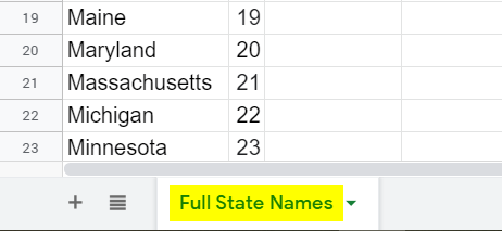
The Tab Name. It’s important not to forget this step. Even if your spreadsheet only has one tab, you still need to include the tab name in the formula or it will not work. This will be added to the formula template. Replace {Tab Name} in the template with the tab name (i.e. Full State Names). When adding this to the formula, it is not case sensitive. Make sure to leave the ! after the tab name in the formula.
The Sheet Range. This is where you will indicate which cells of the spreadsheet you want to capture. You can select only one column or row. You can also select multiple columns. If you plan to add more rows to the spreadsheet, you may want to extend the range completely by selecting the entire column(s). In the example below, if I wanted the entire column, the range would simply be A:B. This will replace the {Sheet Range} portion of the template.

Put it all together. Now that we have collected all of the elements of the formula, you can put them together and they should look something like this:
=IMPORTRANGE("https://docs.google.com/spreadsheets/d/1-20JTlPxAR5mkln8uqumudb-9yTYIQ9S2N-mDIKUcDs/edit#gid=0","Full State Names!A:B") Step 4: Allow Permissions
Once you add this formula to your spreadsheet and hit enter, you’ll notice that it immediately comes up and says #REF!. Don’t worry, this is expected. You simply need to allow permissions for this spreadsheet to read the other spreadsheet and you’ll only need to do this one.
Click on the cell that says #REF! and you’ll see a pop up box that says “You need to connect these sheets”.
Click on the blue Allow Permissions button and you’ll see your content start populating in the spreadsheet.

Now What?
You can arrange your merged data how ever you would like and even use formulas, change the font colors and sizes, and set up conditional formatting on the data.
In the example below, I’ve added column B and D (which are both IMPORTRANGE formulas). Additionally, I have set up a conditional format for column A through E for any numbers between 10 and 20.

I would love to hear about how you’re using this formula for your spreadsheets and how it makes your life easier. Leave a comment below!


I have this set up and it did import the data, but when data is updated it is not syncing and updating the data. Any suggestions?